Predicting Survival on the Titanic

Introduction

RMS Titanic was a British passenger liner that sank on April 15, 1912 on its way to New York. It was perhaps the most infamous shipwreck in world history. The Titanic sank after colliding with an iceberg, killing 1502 out of 2224 people, including passengers and crew. The Titanic data set obtained from Kaggle contains data for only 891 passengers of the Titanic who either survived or died during the disaster. This is a basic Kaggle data set that can be approached with a challenge and creativity. The data set contains the information about age, sex, passengers class, family on-board, ticket number, ticket price, where passengers boarded the ship, and cabin location. The ultimate goal here was to get the highest possible accuracy score and achieve a ranking of top 10% in Kaggle competition.

Analysis Overview and Strategy

To approach the problem of determining who survived or died in the Titanic accident, I broke the analysis into several parts, including an initial exploratory analysis. In the initial exploratory stage, I wanted to detect any possible interactions for defining my statistical model. When features interact, the effect of one independent variable depends on the level of the other independent variables.

For example, intuitively it makes sense to assume that more females survived on the Titanic than males. However, it also makes sense to assume that more females who traveled in 1st class vs. females who traveled in 3rd class survived. That is, if females of 1st class were more likely to survive than females of 3rd class, there is a possible interaction. Another possible interaction is between age and class, and so on. Thus, my first goal was to explore all the possible interactions.

My second goal was to address missing data for the variable Age. About 20% of the total number of observations for Age are missing values, which would leave me with only 712 data points and decrease predictive accuracy of the model. This problem could be addressed by using an advanced imputation method.

Since the data set contain more data on people who perished vs. survived, my third goal was to combat the imbalanced classes using a synthetic minority over-sampling technique. Finally, nested cross-validation was applied to measure and evaluate the predictive performance of the model.

Exploratory Data Analysis

The correlational matrix below explores the relationship between features. Although, correlational matrix is not specifically informative to explore relationship between categorical and continuous features, some minor trends can be detected.

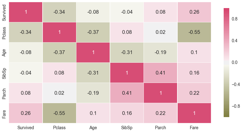
As seen on the matrix, the relationship between features varies from small to moderate. Not all independent variables have significant relationships with the binary outcome Survive, but as I mentioned earlier, correlational matrix is not perfectly informative of a significant relationship between categorical and continuous features.

A set of histograms of continuous features below indicates that normal distribution of Age was slightly skewed towards younger people. The number of younger people (age of 0 to 20) in the data set exceeded the number of elder people (age of 50 and up).

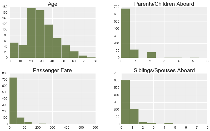
More passengers traveled alone and had neither children, nor parents, nor other family members accompanying them. Most passengers(approximately 70%) paid 50 pounds or less for their fare.

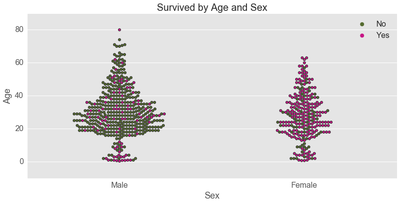
A fist possible interaction between Age and Sex is explored next. Note that each dot on the swarmplot represents a passenger. It looks like age played a significant role in survival of young boys. Age did not seem to play any role in survival of females – females across all ages were more likely to survive on the Titanic.

Second possible interaction was explored between Age and Class.

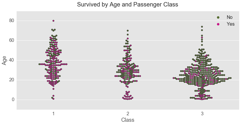
It is obvious from the swarmplot that the passengers of 1st class vs. 2nd and 3rd classes were more likely to survive on the Titanic. However, passengers of infant age were more likely to survive regardless of their class.

The next swarmplot looks into interactive relationships between fare and port of embarkation. In general passengers who embarked in Queenstown were less likely to survive. Also, it seems that proportion wise, passengers who embarked in Cherbourg were more likely to survive.

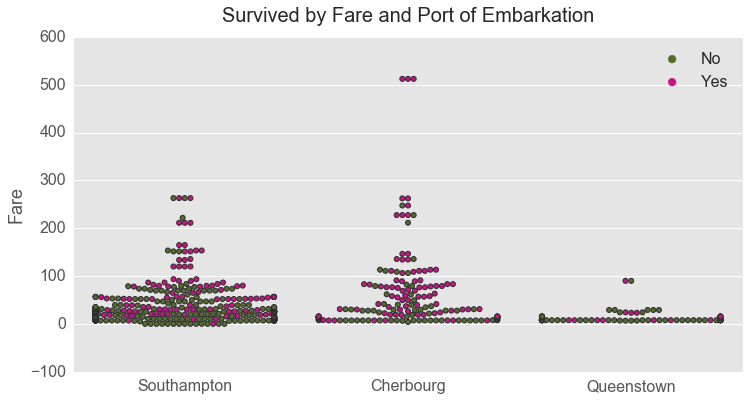
The richest passengers on the ship, who paid the highest fare (over $500) and who embarked in Cherbourg, survived as well. For very rich passengers, gender did not matter whether they survived or not.

Although the three richest passengers on the Titanic survived regardless of their gender, cost of the ticket played a significant role in whether females survived or not.

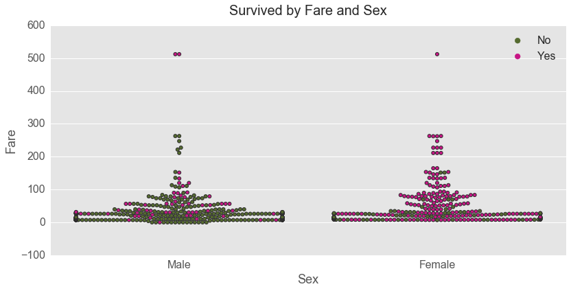
More females who paid a high fare vs. a low fare survived. That was not the case for males. Males were less likely to survive regardless of the fare they paid. It definitely did not pay off to be a male on the Titanic unless that male was super rich.

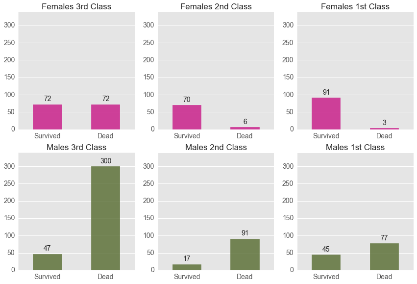
The bar plots below explore the interaction between gender and class. It replicates the findings from the Fare by Sex interaction, but it is another alternative interaction to explore. Females of 1st and 2nd class were more likely to survive, but that was not the case for males. Males were less likely to survive regardless of their class.

Imputation, Random Over-Sampling Technique, and Final Model

Before conducting model selection and evaluation, several imputations were employed to impute missing data for Age. I specifically used several advanced imputation techniques to impute the continuous variable Age since I am a very strong opponent of using mean or median imputation to impute data. It is very bad practice in general as it leads to distortion of the relationship between variables by pulling estimates of the correlation towards zero. Thus, I applied 4 advanced techniques to impute the Titanic data: 1) KNN, 2) Convex Optimization, 3) Spectral Regularization Algorithm, and 4) Multiple Imputations by Chain Equations or MICE

To compare across the imputation algorithms, I used root-mean-square error (RMSE), replicating work by Schmitt, Mandel, and Guedj (2015). This method, however, did not bring me any success as I found no variations in imputation techniques detected by RMSE. Thus, I performed a model comparison (for review see Schmitt, Mandel, & Guedj, 2015) by comparing accuracy scores of various algorithms. See python codes and outputs here. I finally chose the KNN imputation technique as it gave me the highest accuracy scores across the algorithms.

Further, I compared the accuracy scores across various algorithms (Decision Tree, Logistic Regression, Bagging DT, Random Forest, Extra Trees, Ada Boost, Gradient Boosting, Bernoulli NB, and KNN ) and various statistical models (models with/without various interactions) for the imputed data set and for the original data set. My final choice was the statistical model with Fare-by-Sex interaction with KNN imputation and the Gradient Boosting Algorithm.

Finally, I performed a random over-sampling technique. Since more Titanic passengers died than survived, the number of observations belonging to this class was substantially higher than those belonging to the other class. To evaluate and tune my model, I conducted nested cross-validation since it is the best way to evaluate a model when a data set is small. This technique allows to avoid a model’s overfitting (Cawley, & Talbot, 2010).

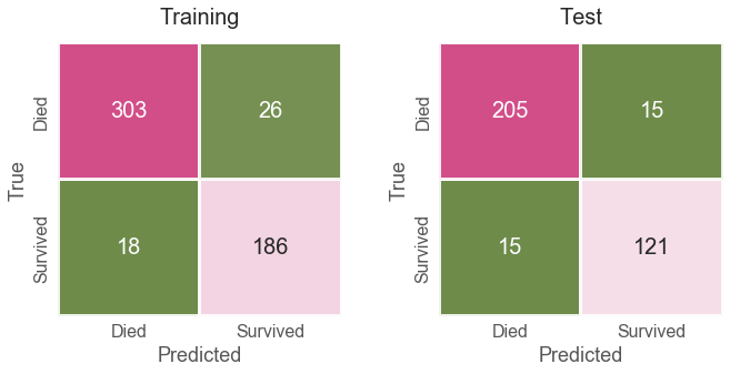
After performing all these techniques, I obtained a 91.74% accuracy score on my training set and 91.57% on my test set. Below are the confusion matrices for training, test, and complete data sets.

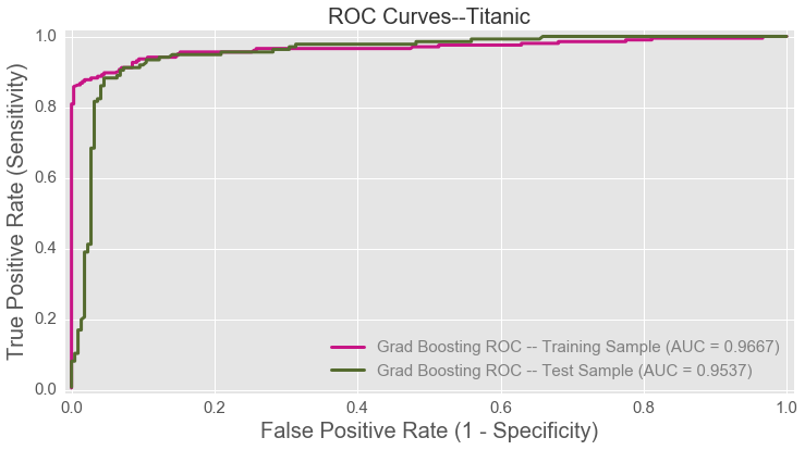
These techniques also helped me yeild very high AUC scores.

Conclusion

Achieving 91.57% accuracy on 40% of the Titanic test data without overfitting is quite good. This would be a top 10% score on the Kaggle board. I don’t think I expected these results using the techniques I did, and I am pleasantly surprised. This high score was achieved using a complex imputation technique, a synthetic minority over-sampling technique (Random Over Sampler), and statistical modeling techniques.